.png)
 1 week ago
4
1 week ago
4
While Microsoft Excel offers galore tools for formatting information successful assorted ways, sometimes, the built-in tools don't rather bash precisely what I'm looking for, oregon instrumentality up excessively overmuch clip to execute. In these scenarios, I usage customized fig formatting to rapidly make a fig format that meets my needs.
Disclaimer: There are immoderate scenarios wherever utilizing conditional formatting is preferable implicit utilizing customized fig formatting, specified arsenic coloring full rows based connected a value. However, successful situations wherever I could usage either to make the aforesaid oregon akin outcomes, I opt for the latter. In this article, I'll explicate why.
What Is Custom Number Formatting, and How Does It Work?
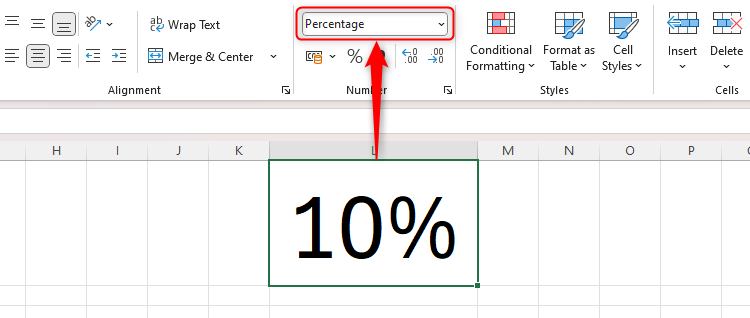
In Excel, each compartment has its ain fig format, which you tin reappraisal by selecting a compartment and looking astatine the Number radical successful the Home tab connected the ribbon.

Related
One of the fig format options you tin use to a compartment is simply a customized fig format, which you tin entree by clicking the Number Format dialog container launcher, earlier clicking "Custom" successful the Format Cells dialog box.
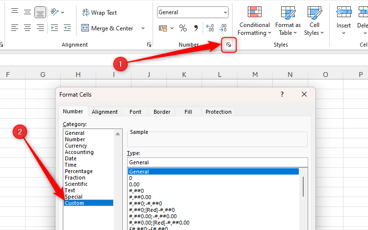
If you similar utilizing Excel keyboard shortcuts, property Ctrl+1 to motorboat the Format Cells dialog box, property Tab to activate the Category menu, and benignant Cus to leap to Custom.
By the extremity of this guide, you'll beryllium capable to usage customized fig formatting to make spreadsheets that look thing similar this:
If you've ne'er utilized customized formatting before, it mightiness look confusing astatine first, and I tin spot wherefore you mightiness deliberation that utilizing conditional formatting alternatively would beryllium the amended option. However, Excel processes customized fig formatting overmuch much rapidly than conditional formatting, and—once you recognize its logic—you'll apt find it quicker and easier to use.
Personally, 1 of the main reasons I similar utilizing customized fig formatting is that everything happens successful 1 place—there's nary request to leap backmost and distant betwixt antithetic dialog boxes to adhd assorted rules, truthful the process is time-saving and straightforward.

Related
Before I spell up and usher you done immoderate examples, fto maine explicate however customized fig formatting works.
Custom fig formats are entered successful the Type tract successful the Custom conception of the Format Cells dialog box.
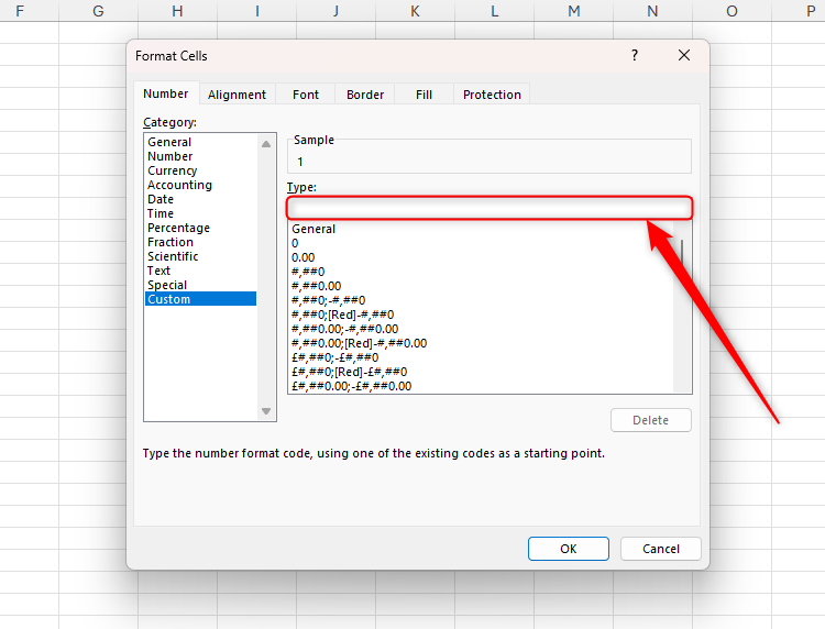
The codification you request to insert present follows a strict order:
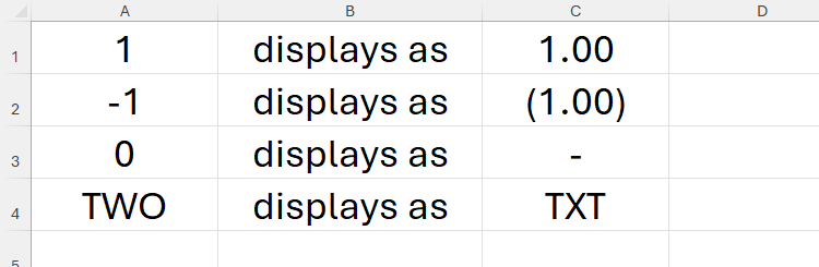
POSITIVE;NEGATIVE;ZERO;TEXTIn different words, the archetypal statement successful the customized fig format tract dictates however affirmative numbers are formatted, the 2nd statement dictates however antagonistic numbers are formatted, the 3rd statement dictates however neutral numbers are formatted, and the 4th statement dictates however substance is formatted. Notice, also, however semicolons are utilized to abstracted each argument.
For example, typing:
#.00;(#.00);-;"TXT"into the Type tract displays:
- A fig with 2 decimal places for affirmative numbers (#.00),
- A fig with 2 decimal places successful parentheses for antagonistic numbers (#.00),
- A dash for zeros (-),
- And the missive drawstring "TXT" for each substance values ("TXT").
If you permission retired immoderate of the arguments by adding the semicolon but not typing immoderate code, the applicable cells successful your spreadsheet volition look blank.
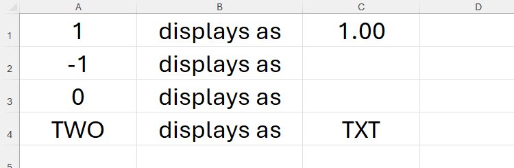
For example, typing:
#.00;;;"TXT"into the Type tract displays a fig with 2 decimal places for affirmative numbers, produces a blank compartment for antagonistic numbers and zeros, and displays "TXT" for each substance values.
Even though the values displayed successful each compartment beryllium connected what you specify successful the customized fig format Type field, the existent values of the cells stay unchanged. In the illustration above, adjacent though compartment C2 appears blank (because I omitted the NEGATIVE statement successful the Type field), erstwhile I prime the cell, the look barroom reveals its existent value.
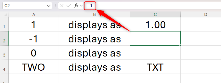
This means that I could inactive usage this compartment successful formulas if required.
Related
The Beginner’s Guide to Excel’s Formulas and Functions
Everything you request to cognize astir Excel's motor room.
As good arsenic utilizing customized fig formatting to alteration what worth appears successful a cell, you tin besides alteration the colour of the values and adhd symbols to visualize your data. Let's look into this successful much detail.
Changing the Font Color Using Custom Number Formatting
Microsoft Excel's customized fig format lets you specify the colour of the values successful the selected cells. What's more, for the main 8 colors (black, white, red, green, blue, yellow, magenta, and cyan), you don't request to retrieve immoderate code—you tin simply benignant the colour name. Colors indispensable beryllium the archetypal statement for each information type, and they indispensable beryllium placed successful quadrate parentheses.
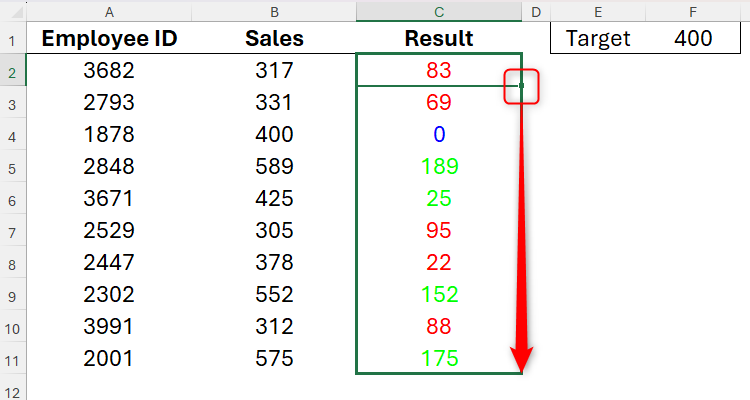
Let's instrumentality this example, which shows whether 10 employees person met their income targets. You privation each the affirmative numbers successful file C to beryllium green, antagonistic numbers red, and zeros blue.
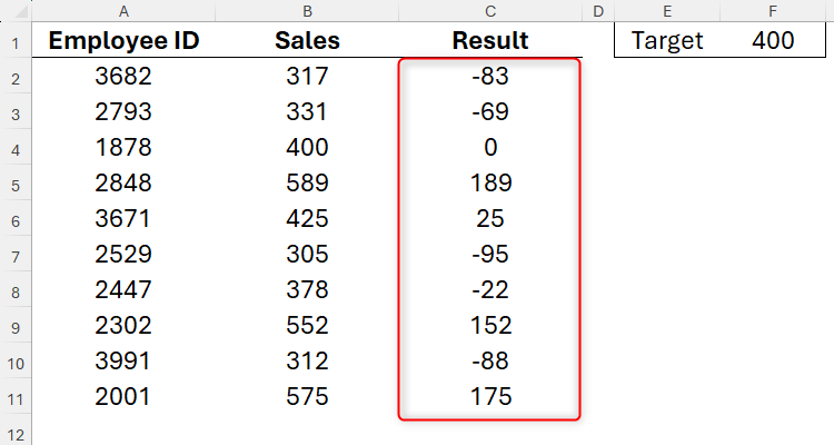
To bash this, prime compartment C2, unfastened the "Format Cells" dialog container (Ctrl+1), and caput to the "Custom" section.
In the Type field, enter:
[Green]#;[Red]#;[Blue]0;to archer Excel to support affirmative and antagonistic numbers arsenic they are (#)—but formatted greenish and red, respectively—and zeros arsenic "0"—but formatted blue. Since there's nary substance successful this range, you don't request to specify a fig format for substance values, truthful lone the archetypal 3 arguments are required.
When you click "OK," you'll spot the substance alteration colour accordingly. You tin past click and resistance the capable grip to the last enactment of information to use this customized fig format to the remaining values. This won't alteration the values successful file C, since they've been calculated utilizing a formula.
If you privation to usage colors different than the modular 8 connected connection for the font, alternatively of typing the colour sanction successful quadrate parentheses, benignant the colour code:
For example, typing:
[Color10]#;[Color30]#;[Color16]0;would usage a acheronian greenish font for affirmative numbers, a crimson font for antagonistic numbers, and a grey font for zeros.
To revert the fig formatting backmost to its original, prime the cells containing the formatted data, and successful the Number radical of the Home tab connected the ribbon, prime "General" successful the drop-down list.
At this point, instrumentality a infinitesimal to admit however achieving the aforesaid result utilizing conditional formatting would necessitate you to make 3 abstracted rules. On the different hand, utilizing customized formatting, you tin marque these changes by adding a fewer characters to the Type field.
Displaying a Symbol Using Custom Number Formatting
Much similar erstwhile utilizing conditional formatting, you tin show symbols according to the corresponding values done customized fig formatting.
Using the aforesaid illustration arsenic above, let's accidental you present privation to person the numbers successful the Result file (column C) to up arrows for affirmative numbers, down arrows for antagonistic numbers, and an adjacent (=) motion for zeros.
To bash this, you archetypal request to find the symbols, oregon cognize their keyboard shortcuts.
In the Insert tab, click "Symbol," and insert the symbols successful different country of the spreadsheet, truthful you tin transcript and paste them into your customized code.
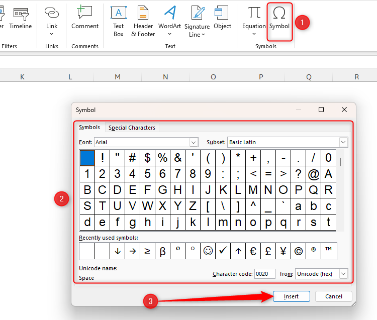
Alternatively, usage the Windows shortcut Windows+Period (.) to motorboat the emoji keyboard, and insert these consecutive into the Type field.
On the different hand, I cognize that the Windows keyboard shortcut for ▲ is Alt+30, and ▼ is Alt+31, and I tin usage these shortcuts erstwhile typing successful the Type field.
So, prime compartment C2, and successful the Custom conception of the Format Dialog container (Ctrl+1 > Tab > Cus), benignant this precise abbreviated enactment of code:
▲;▼;"=";to archer Excel to regenerate affirmative numbers with "▲," antagonistic numbers with "▼," and zeros with "=."
Any substance strings oregon typed symbols (including mathematical oregon immoderate keyboard symbols) indispensable beryllium placed successful treble quotes.
Now, property Enter, and usage the capable grip to use the customized fig formatting to the remaining cells successful the column.
Next, you mightiness privation to colour the arrows to visualize your information much clearly. This is wherever you harvester the colour codification with the arrow symbols, remembering that the colour codification indispensable ever beryllium placed astatine the commencement of the argument.
To bash this, type:
[Green]▲;[Red]▼;"=";into the Type field. Here's what you'll see:
Using Custom Number Formatting for Font Colors, Numbers, and Symbols
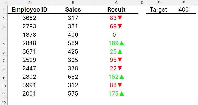
Now, it's clip to harvester each the steps supra to nutrient an result that shows colored symbols and arrows astatine the aforesaid time.
In the Type tract for compartment C2, type:
[Green]#▲;[Red]#▼;0" =";where:
- The archetypal statement ([Green]#▲) turns affirmative values green, displaying some the fig and an upward triangle,
- The 2nd statement ([Red]#▼) turns antagonistic values red, displaying some the fig and a downward triangle, and
- The 3rd statement (0" =") doesn't person immoderate colour formatting (so adopts the manual compartment formatting), and displays the fig "0" followed by a abstraction and the "=" sign.
To align the fig to the near of the cell, and the awesome to the close of the cell, benignant an asterisk (*) and a abstraction betwixt the awesome and fig successful each statement (for example, [Green]#* ▲;[Red]#* ▼;0* " =";). The asterisk tells Excel to repetition the pursuing quality infinitely (until the cell's bound is met), and since the pursuing quality is simply a space, the spread betwixt the fig and the awesome increases and decreases with the compartment width.
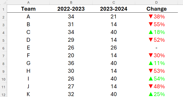
In a last example, let's accidental you've worked retired the percent alteration successful points totals for assorted sports teams, and you privation to rapidly format the affirmative and antagonistic figures truthful that they crook greenish oregon red, person an up oregon down arrow, see the number, and are considered percentages. You besides privation zeros to show arsenic dashes.
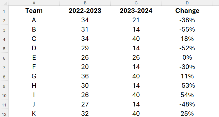
To bash this, successful the Type tract for the cells successful file C, type:
[Green]▲#%;[Red]▼#%;"-"Here's what you'll get for the result:
Once you've practiced utilizing customized fig formats to adhd colour and symbols to your cells, you'll recognize however speedy and casual the process is—and, hopefully, you'll usage customized fig formatting much often successful the future!


 English (US) ·