How to Use Excel's AGGREGATE Function to Refine Calculations

Excel's AGGREGATE relation lets you execute calculations whilst ignoring hidden rows, errors, oregon different functions that look successful the data. It's akin to the SUBTOTAL relation but provides much calculation options and gives you much power implicit what you privation to exclude from the calculation.

The AGGREGATE Syntax

Before we look astatine immoderate examples of the AGGREGATE relation successful use, let's spot however it works. The AGGREGATE relation has 2 syntaxes—one for references and 1 for arrays—though you don't request to get yourself tied up successful knots implicit which 1 you're using, arsenic Excel selects the applicable 1 depending connected the arguments you input. You tin spot some syntaxes successful usage erstwhile I amusement you immoderate examples soon.

The Reference Form Syntax

The syntax for the notation signifier of the AGGREGATE relation is:

=AGGREGATE(a,b,c,d)

where

• a (required) is simply a fig that represents the relation you privation to usage successful the calculation,
• b (required) is simply a fig that defines what you privation the calculation to ignore,
• c (required) is the scope of cells connected which the relation volition beryllium applied, and
• d (optional) is the archetypal of up to 252 further arguments that specify further ranges.

The Array Form Syntax

On the different hand, if you're moving with arrays, the syntax is:

=AGGREGATE(a,b,c,d)

where

• a (required) is simply a fig that represents the relation you privation to usage successful the calculation,
• b (required) is simply a fig that defines what you privation the calculation to ignore,
• c (required) is the array of values connected which the relation volition beryllium applied, and
• d is the 2nd statement required by array functions similar LARGE, SMALL, PERCENTILE.INC, and others.

Functions and Exclusions (Arguments a and b)

When entering arguments a and b successful either syntax signifier above, you'll person assorted options to take from.

The array beneath shows the antithetic functions you tin usage successful the AGGREGATE calculation (argument a). Even though you mightiness beryllium tempted to benignant the relation name, retrieve that this statement indispensable beryllium a fig that represents the relation you privation to use. Functions 1 to 13 are for usage with the notation signifier syntax, and functions 14 to 19 are for usage with the array signifier syntax.

This array lists the numbers you tin input to exclude definite values erstwhile creating your AGGREGATE look (argument b):

Now, let's look astatine immoderate examples of however you tin usage the AGGREGATE relation successful real-world scenarios.

Example 1: Using AGGREGATE to Ignore Errors

This Excel spreadsheet contains a database of shot players, the fig of games they've played, the fig of goals they've scored, and their game-per-goal ratios. Your purpose is to enactment retired the mean game-per-goal ratio for each the players combined.

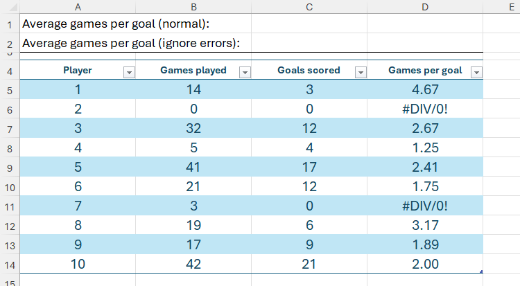
If you were to usage the AVERAGE function unsocial by typing:

=AVERAGE(Player_Goals[Games per goal])

into compartment C1, this would instrumentality an error, due to the fact that the referenced scope contains #DIV/0! errors.

Instead, utilizing the AGGREGATE relation gives you the enactment to disregard these errors and instrumentality the mean for the remaining data. To bash this, successful compartment C2, you request to type:

=AGGREGATE(1,6,Player_Goals[Games per goal])

where

• 1 (argument a) represents the AVERAGE function,
• 6 (argument b) tells Excel to disregard errors, and
• Player_Goals[Games per goal] is the reference.

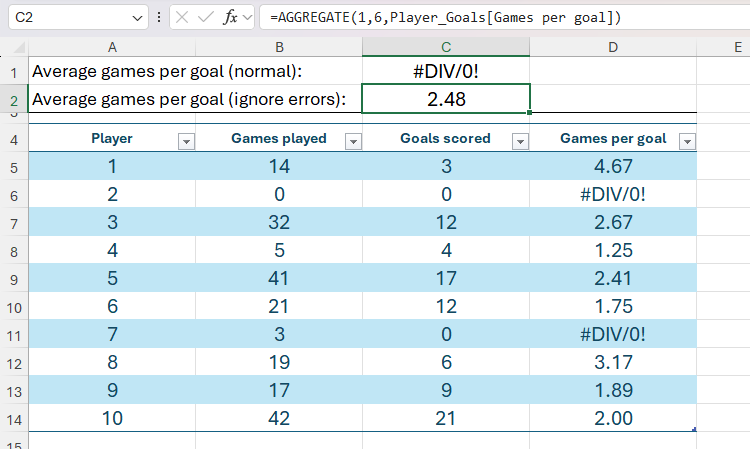
Using the aforesaid spreadsheet, your adjacent people is to cipher the full fig of goals the squad has scored.

Specifically, you privation to show 2 totals. The archetypal is the wide full erstwhile you harvester the goals scored by each players, but the 2nd is the full of lone the players showing successful the array aft you use filters.

To cipher the wide total, successful compartment C1, type:

=SUM(Player_Goals[Goals scored])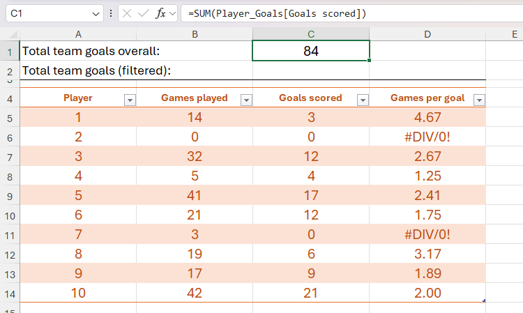

Now, adjacent aft you use a filter to 1 of the columns, specified arsenic displaying lone the players who person played 15 games oregon more, the SUM look you conscionable applied inactive includes the rows that are filtered out.

This is wherever the AGGREATE relation volition prevention the day, arsenic it allows your calculation to disregard rows that are filtered out. In fact, the AGGREGATE relation would besides enactment if you wanted to disregard rows you've hidden by right-clicking the enactment header and clicking "Hide."

In compartment C2, type:

=AGGREGATE(9,5,Player_Goals[Goals scored])

where

• 9 (argument a) represents the SUM function,
• 5 (argument b) tells Excel to disregard hidden rows, and
• Player_Goals[Goals scored] is the reference.

Now, announcement that the effect of this look differs from the effect of the SUM look you utilized successful compartment C1, due to the fact that it considers lone the rows connected display.

​​​​

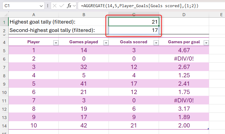
Example 3: Using AGGREGATE to Ignore Hidden Rows (Array)

Next, let's accidental you wanted to database the 2 highest extremity tallies for players who person played 20 games oregon fewer.

You could use the filter archetypal and past make your formula, but for the purposes of this demonstration, let's make the look first.

In compartment C1, type:

=AGGREGATE(14,5,Player_Goals[Goals scored],{1;2})

where

• 14 (argument a) represents the LARGE function,
• 5 (argument b) tells Excel to disregard hidden rows,
• Player_Goals[Goals scored] is the array of values, and
• {1;2} tells Excel that you privation it to instrumentality the largest (1) and second-largest values (2) connected abstracted rows (;).

When you property Enter, announcement that the effect is simply a spilled array covering cells C1 and C2 due to the fact that you told Excel to instrumentality the apical two values.

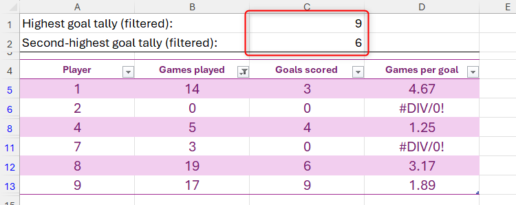
Now, filter the Games Played file to see lone those players who person played 20 games oregon fewer, and spot that the effect of the AGGREGATE look you entered earlier changes to disregard the hidden rows.

Things to Note When Using the AGGREGATE Function

Before you spell up and usage the AGGREGATE relation successful your ain Excel workbooks, instrumentality a infinitesimal to enactment the pursuing pointers:

• Excel's AGGREGATE relation works with vertical ranges only, not horizontal ranges. So, erstwhile you notation a horizontal range, AGGREGATE volition not disregard rows successful hidden columns.
• Argument c successful the AGGREGATE look cannot beryllium the aforesaid compartment oregon scope of cells crossed aggregate worksheets (also known arsenic 3D references).
• Even though the AGGREGATE relation is simply a large mode to bypass errors successful calculations, don't get into the wont of ignoring errors altogether. They're determination for a crushed and could assistance you troubleshoot issues with your data.
• The array signifier of the AGGREGATE relation volition not disregard hidden rows, nested subtotals, oregon nested aggregates if the array statement includes a calculation.

---

Another mode to fell rows successful Excel tables truthful that the AGGREGATE relation lone includes what's showing is by inserting slicers, interactive buttons that you tin click to marque filtering overmuch much straightforward.