How to Format a Spilled Array in Excel

In Excel, you tin use nonstop formatting to cells' values oregon backgrounds to marque the spreadsheet easier to read. However, erstwhile an Excel look returns a acceptable of values—known arsenic a spilled array—applying nonstop formatting volition origin issues if the size oregon signifier of the information changes.

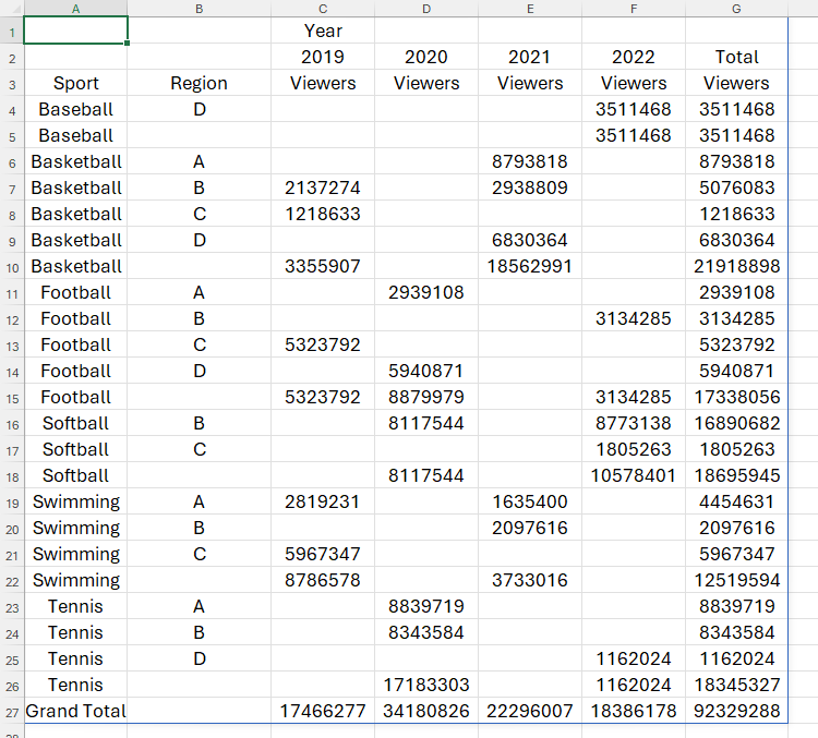
Let's accidental you person this spreadsheet containing the spilled effect of a PIVOTBY formula, which shows the fig of viewers per athletics crossed assorted regions implicit 4 years.

Because the PIVOTBY relation doesn't see an statement that lets you format the result, distinguishing betwixt the header rows, information rows, subtotal rows, and expansive full enactment is difficult.

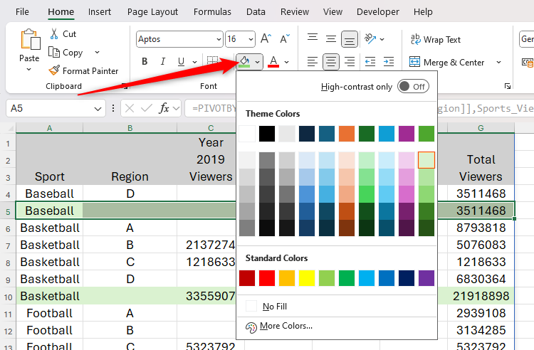
At this stage, you mightiness beryllium tempted to use nonstop formatting—via the Font radical of the Home tab connected the ribbon—to visually abstracted the antithetic types of rows successful the data.

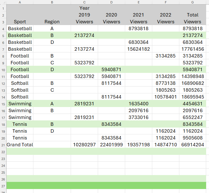
However, if you aboriginal modify the parameters successful the PIVOTBY formula, oregon if the effect grows oregon shrinks owed to changes successful the archetypal data, the nonstop formatting you applied won't set accordingly. This is due to the fact that nonstop formatting successful Excel is linked to the cells, alternatively than the information they contain. See the disorder this could origin successful the screenshot below, wherever the information has shrunk, but the nonstop formatting is inactive applied to the aforesaid rows.

Instead, you should usage conditional formatting, which allows you to format the cells and rows according to their values.

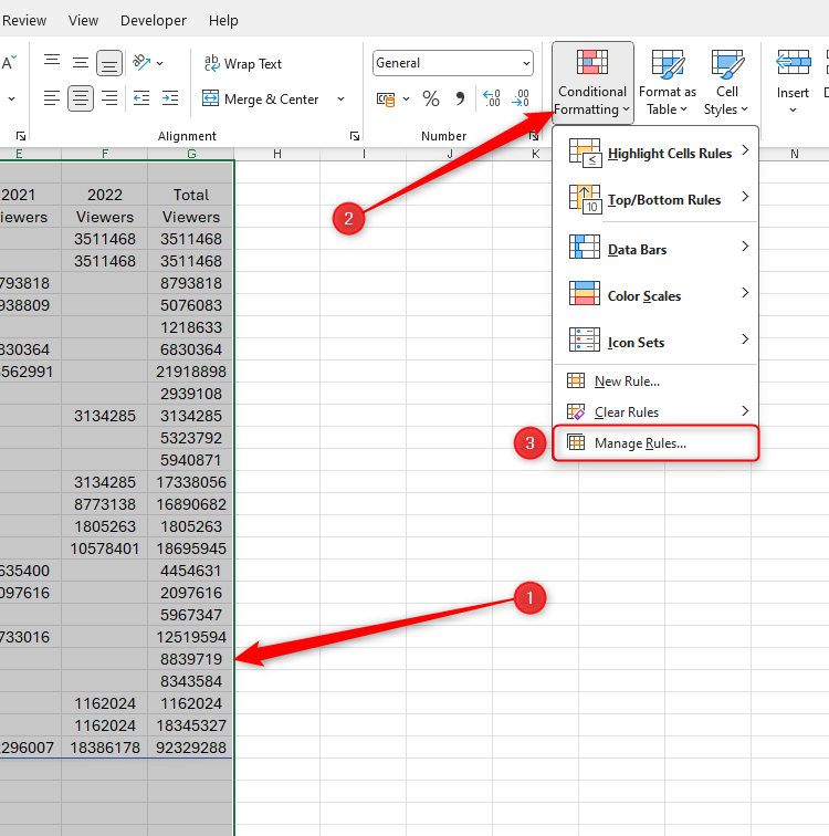
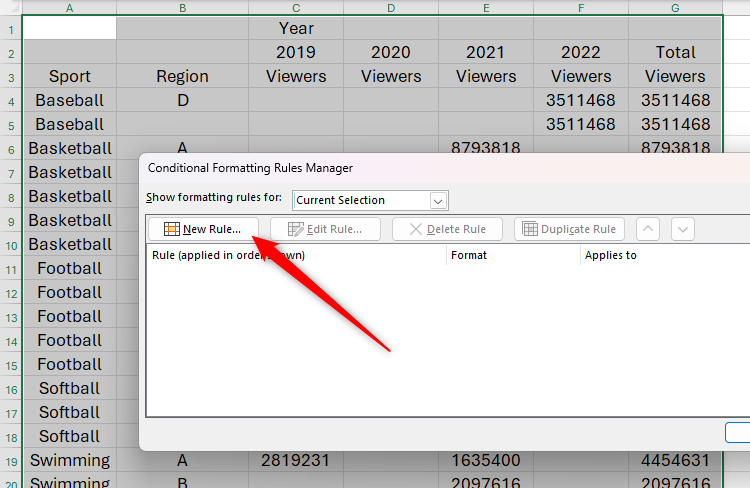
Select each the data—plus immoderate other rows astatine the bottommost to let for vertical growth—and successful the Home tab connected the ribbon, click Conditional Formatting > Manage Rules.

Next, successful the Conditional Formatting Rules Manager dialog box, click "New Rule."

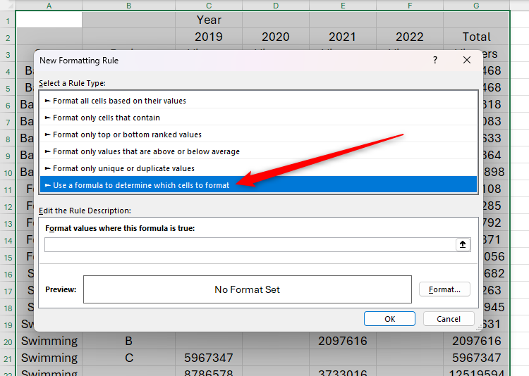
For each of the rules you're going to make to format your spilled array, you'll request to usage a formula. So, successful the Select A Rule Type country of the New Formatting Rule dialog box, prime the last option, "Use A Formula To Determine Which Cells To Format."

The archetypal regularisation you privation to make relates to the header rows. Specifically, you privation those cells to follow a grey background.

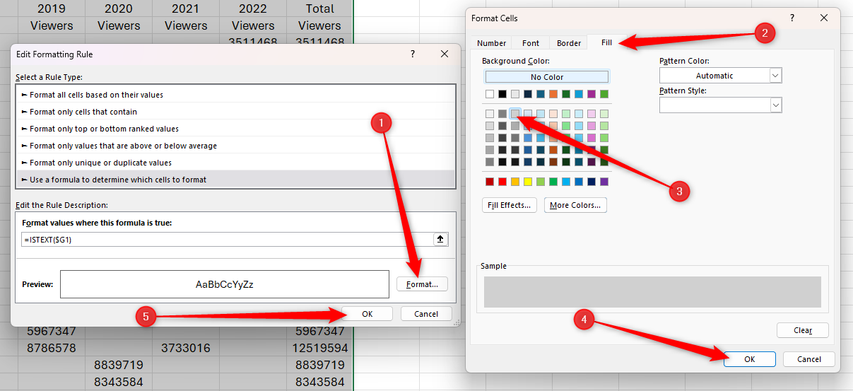
To execute this, instrumentality a infinitesimal to place what makes the header rows unsocial from the different rows successful your table. In this case, the header rows are the lone rows that don't incorporate numbers successful file G. So, successful the look field, type:

=ISTEXT($G1)

Since the ISTEXT function treats blank cells and cells containing substance arsenic a substance value, the conditional formatting regularisation volition see cells G1 to G3 arsenic containing text, with the remaining cells successful file G containing fig values.

Importantly, adding a dollar ($) motion earlier the file reference—also known arsenic a mixed reference—fixes the conditional formatting to this column, portion allowing Excel to use the regularisation to the remaining rows.

Finally, due to the fact that you initially selected information successful columns A to G, the conditional formatting volition use to the full enactment wherever the information is met.

Now, click "Format" to prime the formatting for the header rows. In this case, you privation them to beryllium colored gray. Then, click "OK" successful the Format Cells and Edit Formatting Rule dialog boxes.

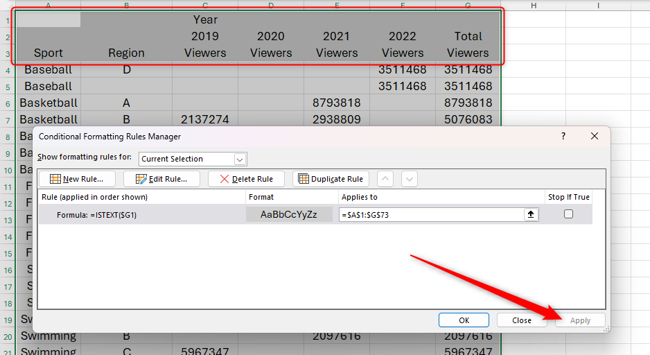
When you click "Apply" successful the Conditional Formatting Rules Manager dialog box, you'll spot that lone the rows successful which file G contains blank cells oregon text—in different words, the header rows—are filled successful gray.

Next, you privation to format the subtotal rows truthful that they follow a airy greenish fill.

Again, cautiously reappraisal the information to spot what conditions you tin usage to use the formatting to these rows only. In this case, the subtotal rows incorporate substance successful file A but thing successful file B. Also, since the expansive full enactment besides meets these criteria, you request to exclude immoderate cells successful file A containing the words "Grand Total."

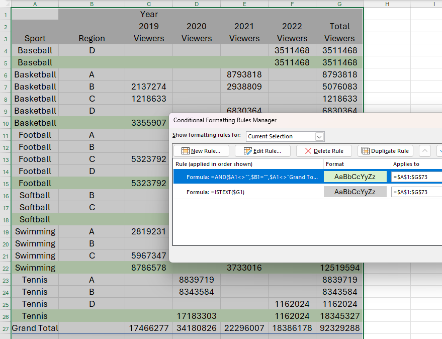
With the Conditional Formatting Rules Manager dialog container inactive open, click "New Rule," and prime the enactment that lets you usage a look to format the cells. This time, successful the look field, type:

=AND($A1<>"",$B1="",$A1<>"Grand Total")

where

• The AND function lets you specify much than 1 information wrong the parentheses,
• $A1<>"" tells Excel to look for cells successful file A that bash not incorporate (<>) blank cells (""),
• $B1="" tells Excel to look for cells successful file B that bash incorporate (=) blank cells (""), and
• $A1<>"Grand Total" tells Excel to exclude (<>) immoderate cells successful file A that incorporate the substance "Grand Total."

As with the erstwhile rule, retrieve to insert the $ motion earlier the file references to let Excel to use the aforesaid regularisation down each the selected rows.

Now, click "Format" to take the airy greenish capable color, and aft closing the Format Cells and Edit Formatting Rule dialog boxes, click "Apply" to spot the subtotal rows filled successful airy green.

Finally, you privation the cells successful the expansive full enactment to beryllium filled with a bolder green.

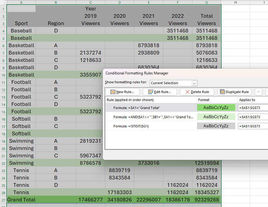
Since the expansive full enactment is the lone enactment that contains the words "Grand Total" successful file A, this is the criterion you tin usage for the conditional formatting. In the Conditional Formatting Rules Manager dialog box, click "New Rule," and prime the last enactment successful the Select A Rule Type list. Now, successful the look field, type:

=$A1="Grand Total"

Next, click "Format," and prime a bold greenish capable colour to use to the cells that lucifer this criterion. Now, erstwhile you adjacent the Format Cells and Edit Formatting Rule dialog boxes, and click "Apply" successful the Conditional Formatting Rules Manager dialog box, you'll spot that your expansive full enactment has adopted this formatting.

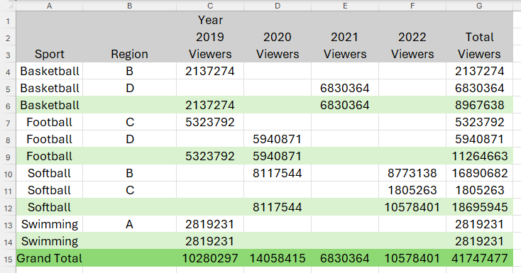
Now that you've applied each your rules, click "Close" successful the Conditional Formatting Rules Manager dialog box. Then, set immoderate of your information successful the archetypal table, and spot the spilled effect and its formatting update accordingly.

In this example, adjacent though I removed 12 rows from the archetypal information table, the spilled PIVOTBY effect is inactive correctly formatted, with the header rows colored gray, the subtotal rows colored airy green, and the expansive full enactment colored bold green.

---

If you request to marque immoderate changes to the rules you person created and applied, simply prime immoderate compartment successful the data, and click Conditional Formatting > Manage Rules to relaunch the Conditional Formatting Rules manager. Then, double-click a regularisation to alteration its conditions.