.png)
 1 week ago
6
1 week ago
6
When I learned however to usage tables successful Microsoft Excel, it wholly transformed however I enactment with data. Even if you deliberation you already cognize everything determination is to cognize astir Excel tables, hopefully, you'll prime up immoderate further tips successful this guide!
Convert Data Into an Excel Table
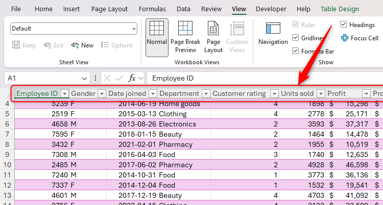
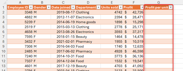
Before you person your Excel information into a table, marque definite you person file headers on the apical row. This volition marque dealing with and utilizing the information overmuch much straightforward down the line.
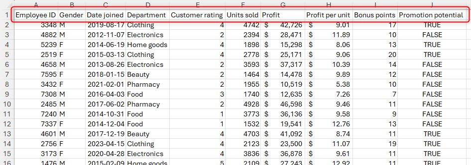
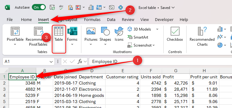
Then, prime each the cells you privation to convert, including your file headers. Alternatively, if your scope is contiguous (in different words, each the cells are adjacent to each different with nary blank columns oregon rows), simply prime 1 compartment successful the data. Then, successful the Insert tab connected the ribbon, click "Table," oregon usage the Microsoft Excel keyboard shortcut, Ctrl+T.

Related
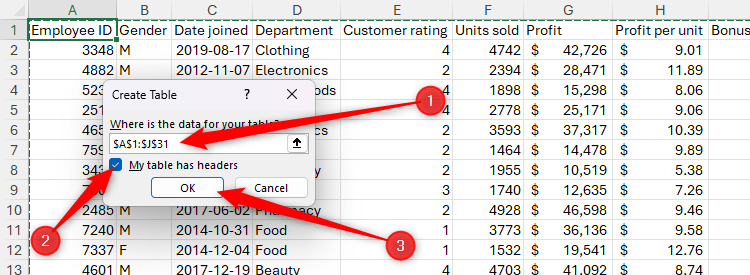
Now, successful the Create Table dialog box, double-check that the full scope is selected, marque definite "My Table Has Headers" is checked, and click "OK."
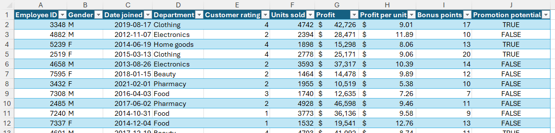
Your information is present a formatted Excel table, with filter buttons added to your file headers.
Change the Table Design
Once your array is created, it's clip to set its layout. When you prime immoderate compartment successful your recently created table, the Table Design tab appears connected the ribbon. Open this tab to spot the antithetic options.
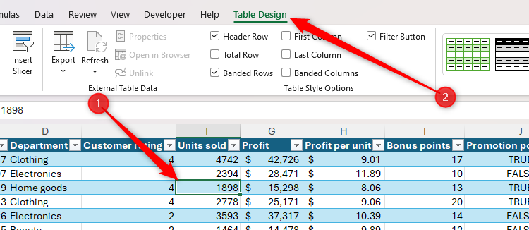
First, click the down arrow successful the Table Styles radical to take from the antithetic layout options. In my case, I've gone for the mean plum style.
Next, caput to the Table Style Options radical successful the Table Design tab to spot respective checkboxes.
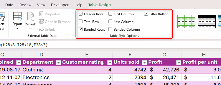
- Header Row: If you checked "My Table Has Headers" successful the Create Table dialog box, permission Header Row checked.
- Total Row: Checking this enactment adds an other enactment to the bottommost of your array wherever you tin adhd file totals (more connected this soon).
- Banded Rows: Enable this enactment to marque it easier to work crossed the table's rows. This is particularly utile if you person tons of columns.
- First Column: This applies formatting to the left-most file successful your table, fundamentally turning this file into enactment headers.
- Last Column: This applies formatting to the right-most file successful your table, which is useful if it contains wide oregon summary figures.
- Banded Columns: Check this enactment to assistance radical travel columns downward. I would counsel that you cheque either Banded Rows or Banded Columns—checking some could origin disorder and marque the array look untidy.
- Filter Button: This enactment adds filter arrows to the header row.
After checking "Total Row," determine which columns you privation to beryllium totaled by selecting the applicable compartment successful the full row, clicking the down arrow, and selecting 1 of the aggregation options.
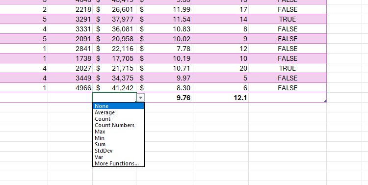
If you use a filter to 1 of the columns, lone the values connected show successful the array volition lend to the totals successful the full row.
The last accommodation you should marque successful the Table Design tab is to springiness your array a name. By default, Excel tables are called Table1, Table 2, Table3, and truthful on. However, changing the array sanction makes your spreadsheet much navigable, helps radical utilizing surface readers, and makes formulas easier to recognize if they notation information successful the table.
Related
To rename a table, caput to the Properties radical of the Table Design tab, and regenerate the default sanction with thing much relevant.
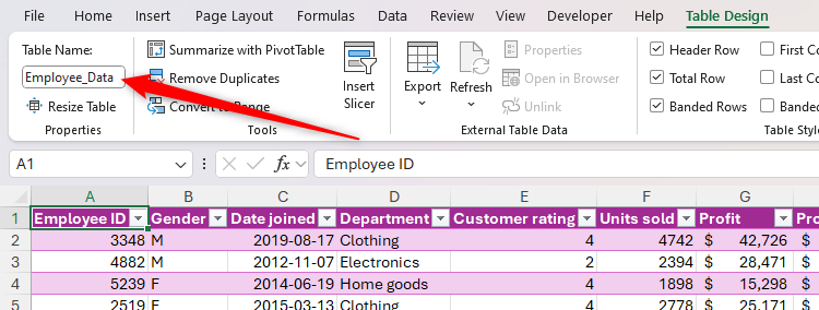
Table names indispensable commencement with a letter, underscore, oregon backslash, with the remaining characters being letters, numbers, periods, oregon underscores. They indispensable besides beryllium unique, can't incorporate a space, and mustn't person the aforesaid sanction arsenic an existing compartment reference, similar A1.
Don't Freeze the Top Row
When moving with ample datasets successful Excel, you mightiness beryllium utilized to freezing the apical row, truthful that erstwhile you scroll down, the file headers stay visible.
However, 1 of the galore benefits of formatting your information arsenic an Excel array is that you don't person to instrumentality this step. Instead, providing you checked "My Table Has Headers" successful the Create Table dialog container and 1 of the cells successful the array is selected, erstwhile you scroll down, the letters supra your spreadsheet that correspond the columns (A, B, C, and truthful on) automatically crook into your array file headers. This works adjacent if the file headers aren't successful the archetypal row.
Notice, also, however these file headers besides show the filter buttons, meaning you don't person to scroll to the apical of your worksheet to alteration what your array displays.
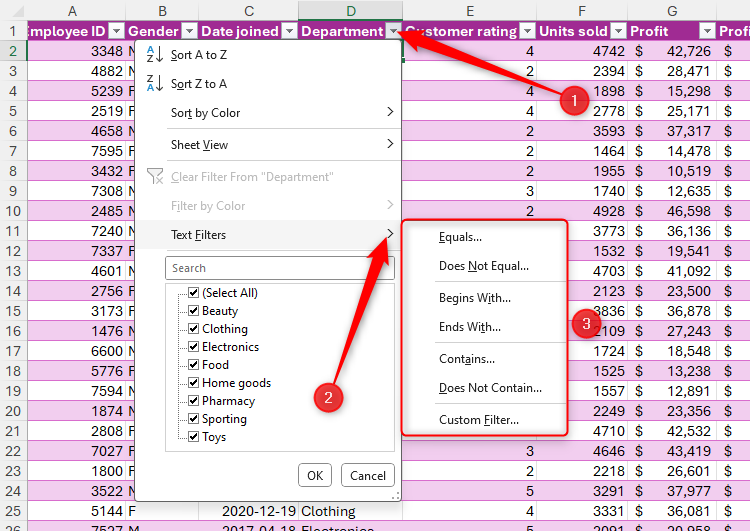
Use the Filter Buttons
I've already mentioned the filter buttons successful Excel tables respective times successful this guide, and that's due to the fact that they're a existent time-saver. In short, the filter buttons marque it casual to constrictive your information to the astir applicable information, redeeming you from having to hunt done your rows and columns manually.
The filter buttons springiness you antithetic options depending connected the benignant of information you person successful each column. For example, the filter fastener for file D—which contains text—offers assorted substance filters, similar searching for values that statesman oregon extremity with definite characters.
On the different hand, erstwhile I click the filter fastener successful a file containing numbers, the filters alteration accordingly.
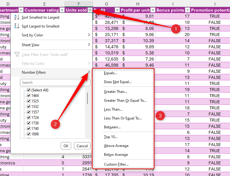
As good arsenic the options to benignant a file successful ascending oregon descending bid oregon filter by color, there's besides a hunt tract successful the filter drop-down, which helps you velocity up the filtering process adjacent further.
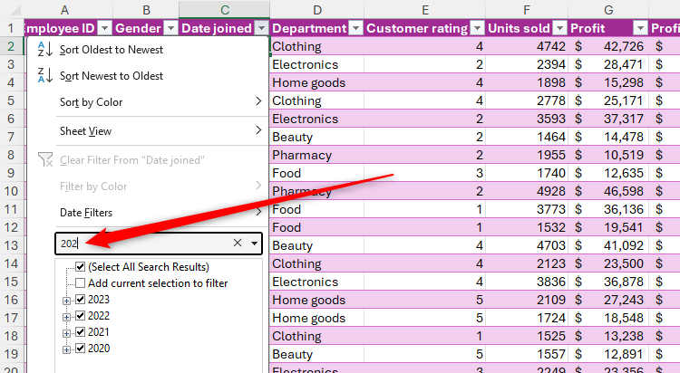
Click "OK" erstwhile you person typed your filter hunt query and checked oregon unchecked the applicable options to use the filter.
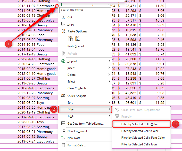
Another nifty instrumentality is to filter a file based connected a selected value. In this example, I lone privation to show employees successful the electronics department. To bash this, I tin right-click a compartment containing the connection "Electronics," and successful the Filter menu, click "Filter By Selected Cell's Value."
Filter With Slicers
While the filter buttons are large ways to signifier and put your data, an adjacent easier mode to bash this is by adding slicers, particularly if a peculiar file is much apt to beryllium filtered than the others.

Related
How to Create Slicers successful Microsoft Excel
Slicers are fun-to-use filter tools for your spreadsheets!
In this example, let's accidental the CEO is astir funny successful the nett made by employees successful antithetic departments and which radical are the champion candidates for promotion. You tin marque the CEO's beingness overmuch easier by adding slicers for these 3 columns.
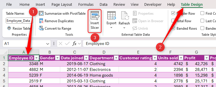
With immoderate compartment successful the array selected, click "Insert Slicer" successful the Table Design tab connected the ribbon.
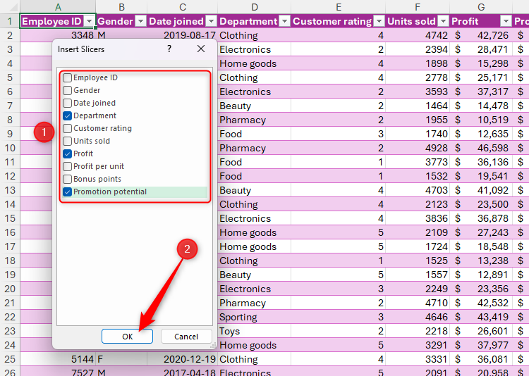
Next, cheque the columns for which you privation to adhd slicers, and click "OK."
Now, click and resistance the slicers to reposition oregon resize them, oregon unfastened the "Slicer" tab connected the ribbon to spot much options. You tin besides right-click a slicer and click "Slicer Settings" to further customize this precocious filtering tool.
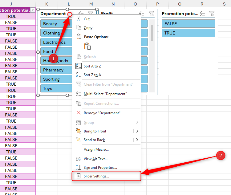
You and your CEO tin present usage the slicers to rapidly filter information successful the Excel table. In this example, the slicers are acceptable to show employees successful the quality and covering departments who person the imaginable for promotion to a higher role, and due to the fact that those selections are colored blue, it's casual to spot however the information is filtered.
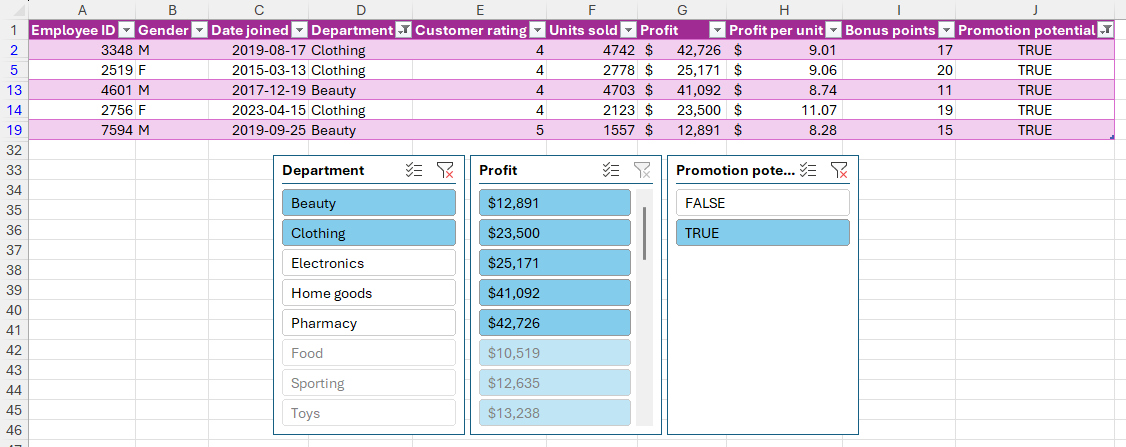
Hold Ctrl erstwhile selecting elements successful a slicer to show them each astatine the aforesaid time, oregon property Alt+C to wide each selections successful the slicer.
Add Columns and Rows
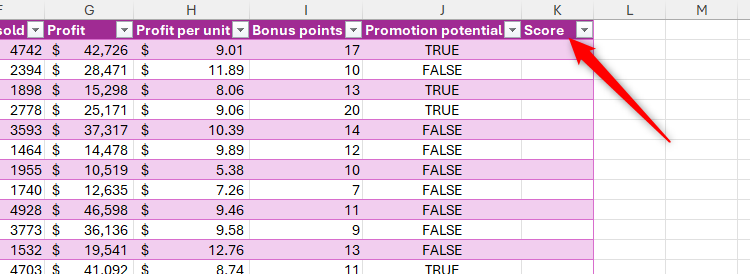
Adding a file to the close oregon a enactment to the bottommost of a formatted Excel array is satisfyingly simple. In this example, arsenic soon arsenic I typed "Score" into compartment K1 and pressed Enter, Excel expanded the table's dimensions to seizure the caller column. This means I don't request to use immoderate manual formatting to the caller data.
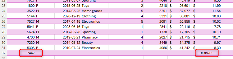
Similarly, erstwhile I added different worker ID to compartment A32, not lone did Excel grow the array downwards, but it besides duplicated immoderate formulas I had created successful erstwhile rows.
If you similar to hole the caller columns and rows before adding the data, click and resistance the table's capable grip close oregon downward. If you usage this method, retrieve to sanction each caller file by adding a header successful the archetypal row.
You tin besides adhd a caller enactment oregon file betwixt existing information by right-clicking the enactment oregon file header, and clicking "Insert," harmless successful the cognition that the array formatting volition beryllium applied automatically to these caller information introduction points.
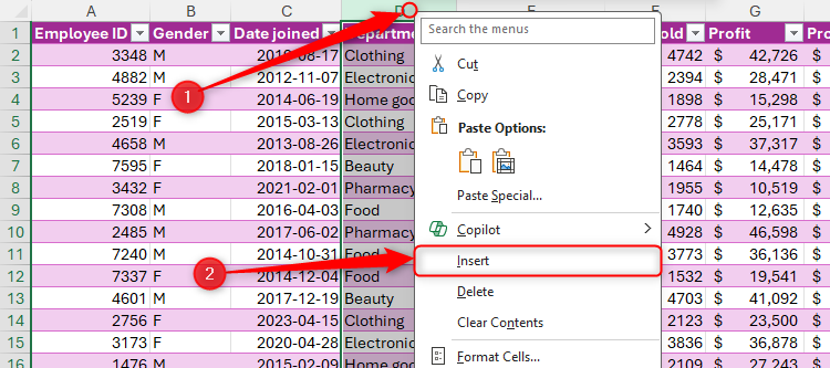
Clicking "Insert" connected a file adds a caller file to the left, portion clicking "Insert" connected a enactment adds a caller enactment above.
Make Column-Based Calculations
Another payment of formatting your information arsenic an Excel array is that performing calculations betwixt the columns becomes overmuch easier and quicker.
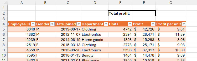
Let's presume you person the array successful the screenshot below, and your purpose is to cipher the nett per portion by dividing the values successful the Profit file by the values successful the Units Sold column.
To bash this, successful compartment G2, benignant =, prime compartment F2, benignant a guardant slash (/), and prime compartment E2. As you bash this, announcement however Excel inserts the file headers—also known arsenic structured references—into your formula, alternatively than nonstop compartment references, and this is wherefore it's important to person named file headers successful your table:
=[@Profit]/[@[Units sold]]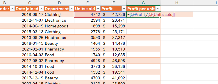

Related
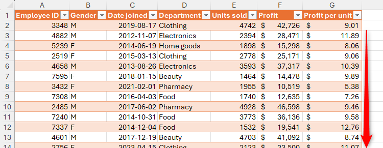
The quadrate parentheses are Excel's mode of indicating that it's utilizing a structured reference, and the @ awesome (also known arsenic the intersection operator) means that the calculation volition beryllium applied respectively to each enactment wrong the table.
When you property Enter, the remaining cells successful the Profit Per Unit file follow the formula.
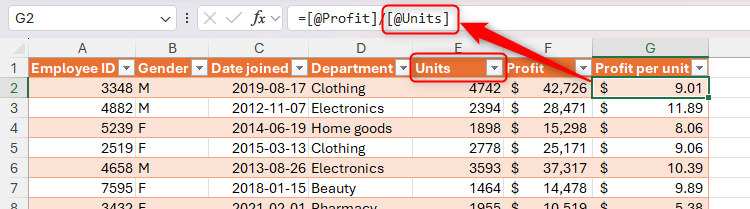
Structured references are easier to create, read, and parse than nonstop references, and they stay loyal to the applicable columns, adjacent if other columns are added. What's more, due to the fact that the full file is referenced successful the look by its header, the calculation volition automatically use to immoderate caller rows you add.
Even much impressively, if you rename 1 of the file headers, the structured notation adapts to accommodate this change. In this example, the Units Sold file has been renamed "Units," and the look successful the Profit Per Unit file reflects this update.
Structured references enactment whether you're moving wrong oregon extracurricular the table, meaning you tin easy notation the array and its columns from anyplace successful the workbook.
Here, I've inserted other rows supra my table, arsenic I privation to cipher the full nett present alternatively than astatine the bottommost to debar having to scroll down each time. Another payment of performing this calculation extracurricular the array is that it ignores immoderate filters. This means I could take to insert a full enactment astatine the bottommost that calculates lone what is displayed and a expansive full extracurricular the array that calculates each the data.
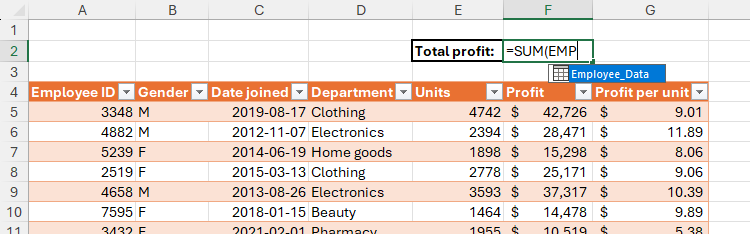
Now, successful compartment F2, I volition type:
=SUM(Then, erstwhile I hover my cursor implicit the Profit file header, it turns to a achromatic down arrow, indicating that it's acceptable to prime the full column.
At this point, erstwhile I click, Excel volition adhd a structured file notation to the formula. However, this time, due to the fact that the look is extracurricular the table, it besides references the array sanction (Employee_Data):
=SUM(Employee_Data[Profit]This is wherefore it's important you sanction your array successful the Properties radical of the Table Design tab connected the ribbon. When I adjacent the rounded parentheses and property Enter, the calculation is complete.
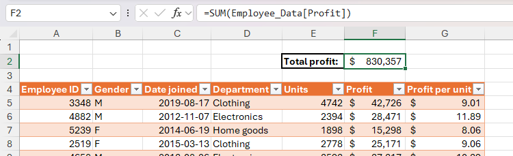
To debar utilizing your rodent successful this process, aft typing =SUM(, commencement typing the array name, and property Tab erstwhile it appears successful the tooltip list.
Then, with the array sanction added to the formula, adhd a quadrate bracket to spot a database of the columns successful the table, usage the arrow keys to prime the applicable label, and property Tab again to adhd it to the formula.
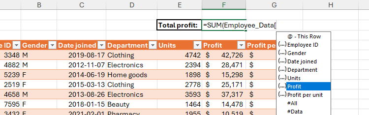
Finally, adjacent the quadrate and rounded parentheses, and property Enter.
Once you've created your table, you tin spell 1 measurement further and convert it into a PivotTable to set however the information is visualized, make broad information summaries, and perform analyzable analyses. What's more, you tin past nutrient PivotCharts, useful if you're looking to create a dashboard containing each your cardinal show indicators.


 English (US) ·